September 26, 2025
The Gambler's Problem
I recently got nerd-sniped[1] by the "Gambler's Problem" in Sutton & Barto's "Reinforcement Learning" book[2]. The problem statement can be described as follows:
A gambler is making bets on a sequence of coin flips. If the coin comes up as heads, he wins as many dollars as he has staked on the flip, if it is tails he loses his stake. The game ends when the gambler reaches his goal of $100, or when he loses by running out of money. On each coin toss, the gambler needs to decide how much of his existing capital he is willing to stake (an integer number of dollars). They can play as many turns as they wish as long as they don't run out of capital. What is the optimal sequence of stakes the gambler should make in order to reach his goal of $100?
Crucially though, we're dealing with an unfair coin, i.e. the probability of getting heads is #(p_H = 0.4)#.
When I first read the problem statement, my thinking was that this sounds trivial: You probably want to always bet the maximum available capital, so you get to $100 as quickly as possible. So if you have a capital of $20, you would stake the full $20. Similarly, if you have a capital of $90, you stake $10 so you get to $100.
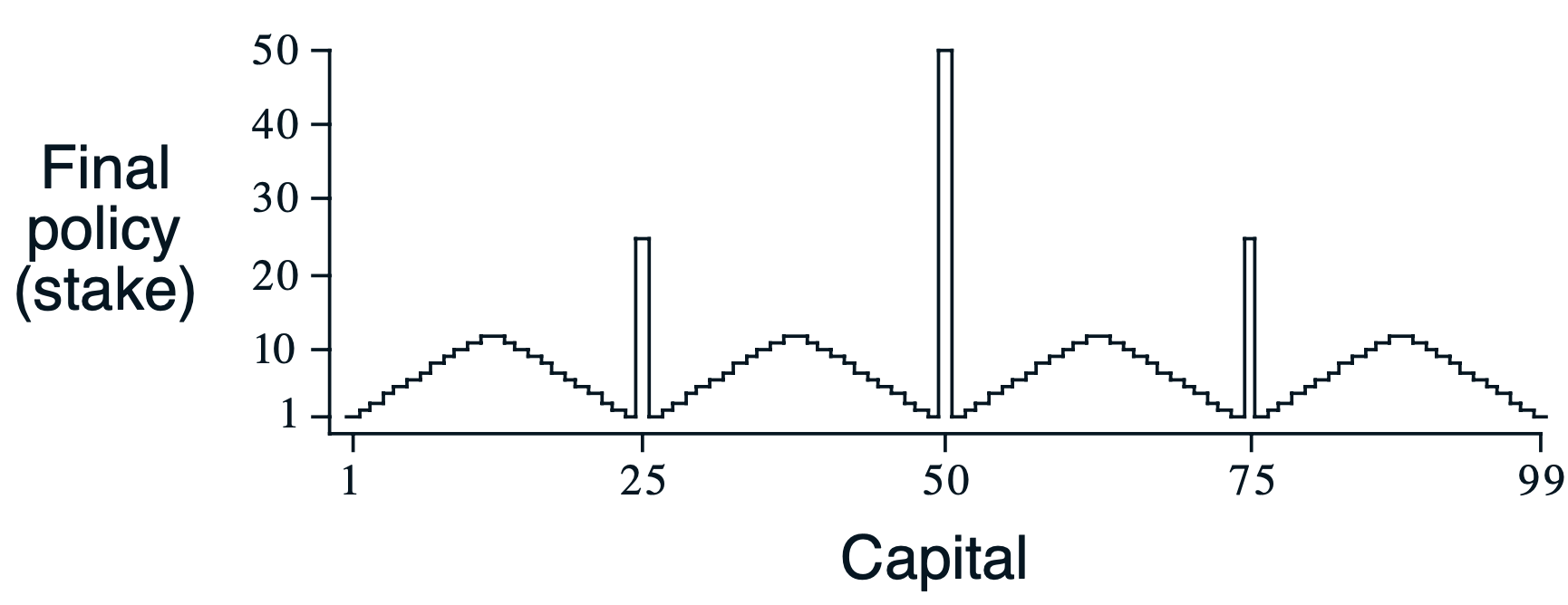
Unexpectedly, the book presents us with a curious looking solution where in most situations we are prudent and only go all-in on certain "strategic" points (most prominently $25, $50, and $75). How can this be? Why go all-in at $50, but bet only $1 at $51? What is so special about these points?
All of this led me down a bit of a rabbit hole. I avoided reading other solutions online, so my path to this is a rather uninformed one, but I did find some insightful things on the way.
Gambling as a reinforcement learning problem
The gambler’s problem is a case of a reinforcement learning problem where we have a finite number of states and a fully known environment model (we know all transition probabilities and rewards). The solution we seek is the optimal policy: the best action to take in any given state. Using the value iteration algorithm is one way we can compute the optimal policy for this problem. Note that our system is stationary and therefore the optimal policy is static.
The states #(S={0, 1, ..., 100})# are the possible capital amounts the gambler could own. Note that 0 and 100 are terminal states, ending the game when reached. The possible actions are #(A={0, 1, ..., \text{min}(s, 100-s)})#, integer amounts of dollars. The gambler cannot bet more than their current capital and they need to reach the target of $100 exactly (they cannot overshoot). In the original version of the problem, we give +1 reward for reaching state 100, and 0 reward for every other state transition. Also note that the gambler may choose to bet $0.
The value iteration algorithm estimates the value of each state. The value tells us how good a state is, i.e. the total expected reward. Knowing the optimized values means we can also derive the optimal policy. It can simply be computed by selecting the action that yields the state with maximal value. However, from any state there may be multiple equally good actions to take, and as such, multiple different optimal policies may exist.
Value iteration repeatedly updates each state's value by taking the maximum over all possible actions of the expected immediate reward plus the discounted future value, until values converge. For this problem, we choose not to discount future rewards since the game has a finite horizon and there's no reason to prefer immediate rewards over future ones.
Reproducing the thing
In order to understand how this pattern emerges, I went ahead and came up with an initial implementation.
import numpy as np
import matplotlib.pyplot as plt

P_HEAD = .4            # unfair coin
DISCOUNT_FACTOR = 1.0  # we choose not to discount future rewards
NUM_STATES = 101       # we include both 0 and 100 as states
THETA = 1e-9           # convergence threshold

def main():
    values = np.zeros(NUM_STATES, dtype=np.float32)
    policy = np.zeros(NUM_STATES, dtype=np.int32)
    it = 0
    while True:
        it += 1
        delta = 0
        for state in range(NUM_STATES):
            if state in [0, 100]:
                # these states are terminal, i.e. we don't optimize them
                continue
            possible_actions = range(min([state + 1, 100 - state + 1]))  # gives e.g. [0, 1, ..., min(s, 100 - s)]
            old_value = values[state]
            for action in possible_actions:
                # we compute the value sum over all possible state transitions (i.e. throwing head or tail)
                # 1. case: head
                head_state = state + action  # we win our stake
                assert head_state <= 100
                head_reward = 1 if head_state == 100 else 0  # only give +1 reward in case of reaching $100
                head_val = P_HEAD * (head_reward + DISCOUNT_FACTOR * values[head_state])
                # 2. case: tail
                tail_state = state - action  # we lose our stake
                tail_reward = 0  # reward will always be zero
                assert tail_state >= 0
                tail_val = (1 - P_HEAD) * (tail_reward + DISCOUNT_FACTOR * values[tail_state])
                new_value = tail_val + head_val
                if new_value > values[state]:
                    # we have found a better value/policy
                    values[state] = new_value
                    policy[state] = action
            # keep track of largest diversion from original value
            delta = max(delta, abs(old_value - values[state]))
        print(f'Iteration: {it:>02}: Delta {delta:.9f}')
        if delta <= THETA:
            break
Which converges in 23 iterations:
Iteration: 01: Delta 0.953343987
Iteration: 02: Delta 0.368896037
Iteration: 03: Delta 0.139264017
Iteration: 04: Delta 0.055705607
Iteration: 05: Delta 0.022282243
Iteration: 06: Delta 0.008912898
Iteration: 07: Delta 0.001638400
Iteration: 08: Delta 0.000393216
Iteration: 09: Delta 0.000076026
Iteration: 10: Delta 0.000030410
Iteration: 11: Delta 0.000002641
Iteration: 12: Delta 0.000000905
Iteration: 13: Delta 0.000000078
Iteration: 14: Delta 0.000000060
Iteration: 15: Delta 0.000000119
Iteration: 16: Delta 0.000000030
Iteration: 17: Delta 0.000000030
Iteration: 18: Delta 0.000000015
Iteration: 19: Delta 0.000000015
Iteration: 20: Delta 0.000000007
Iteration: 21: Delta 0.000000004
Iteration: 22: Delta 0.000000004
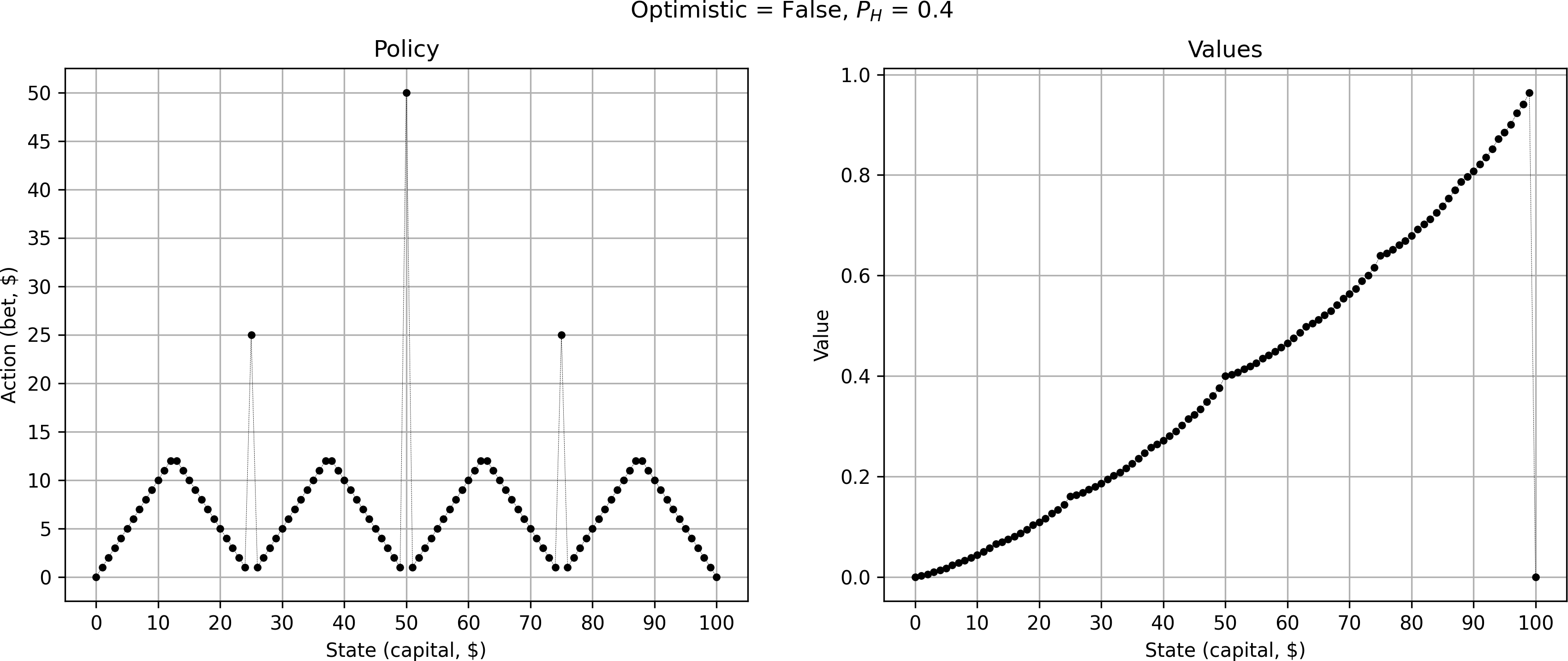
Iteration: 23: Delta 0.000000001Although the value curve looks correct (showing characteristic changes in curvature at points 25, 50, and 75), the resulting optimal policy looked very noisy, very much unlike the iconic graph in the Sutton & Barto book:
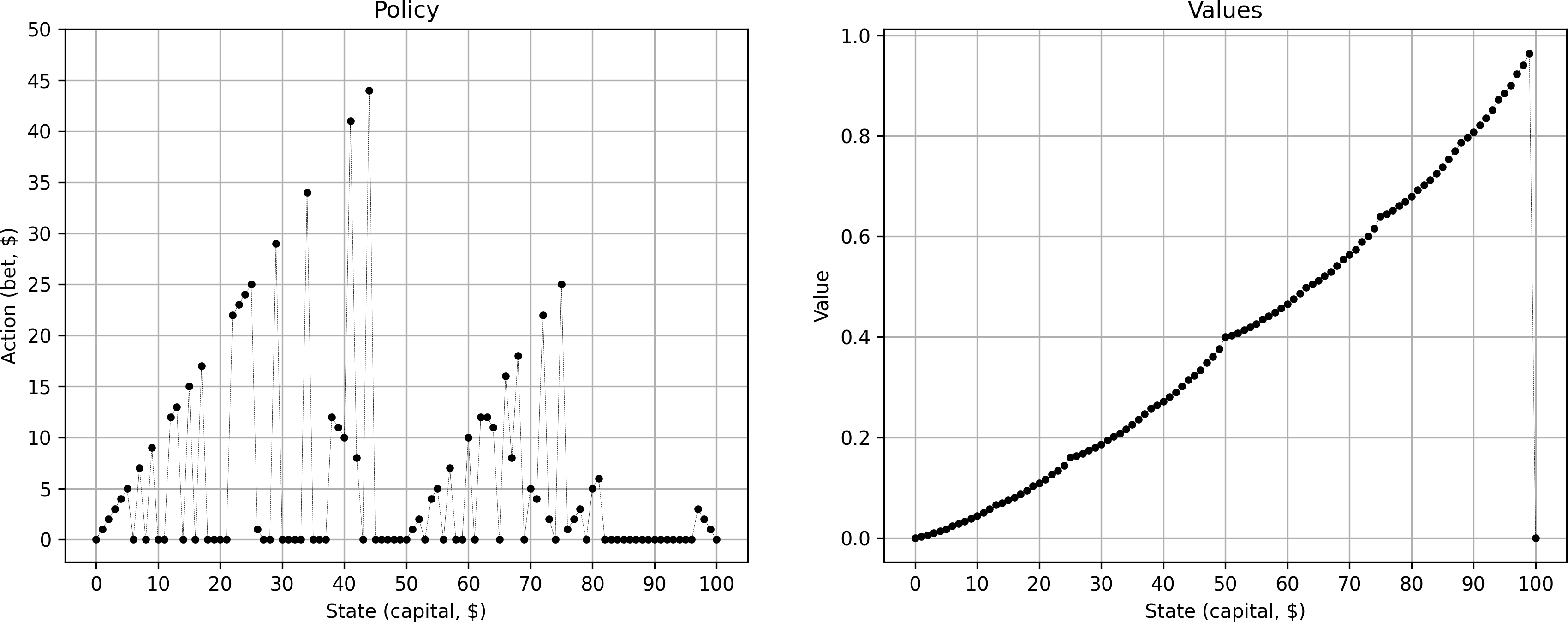
What's more, for many states, the best option for the gambler was to bet 0. Given the coin is rigged, not playing at all seems indeed to be the wisest choice. However, given the framing of the problem, we are committed to play and not betting anything is not an interesting option. We change the code to avoid tracking action 0 from our best policy:
-                    policy[state] = action
+                    if action > 0:
+                        policy[state] = action
This gives something that looks already a lot closer — we are now starting to see the typical “sawtooth” pattern.
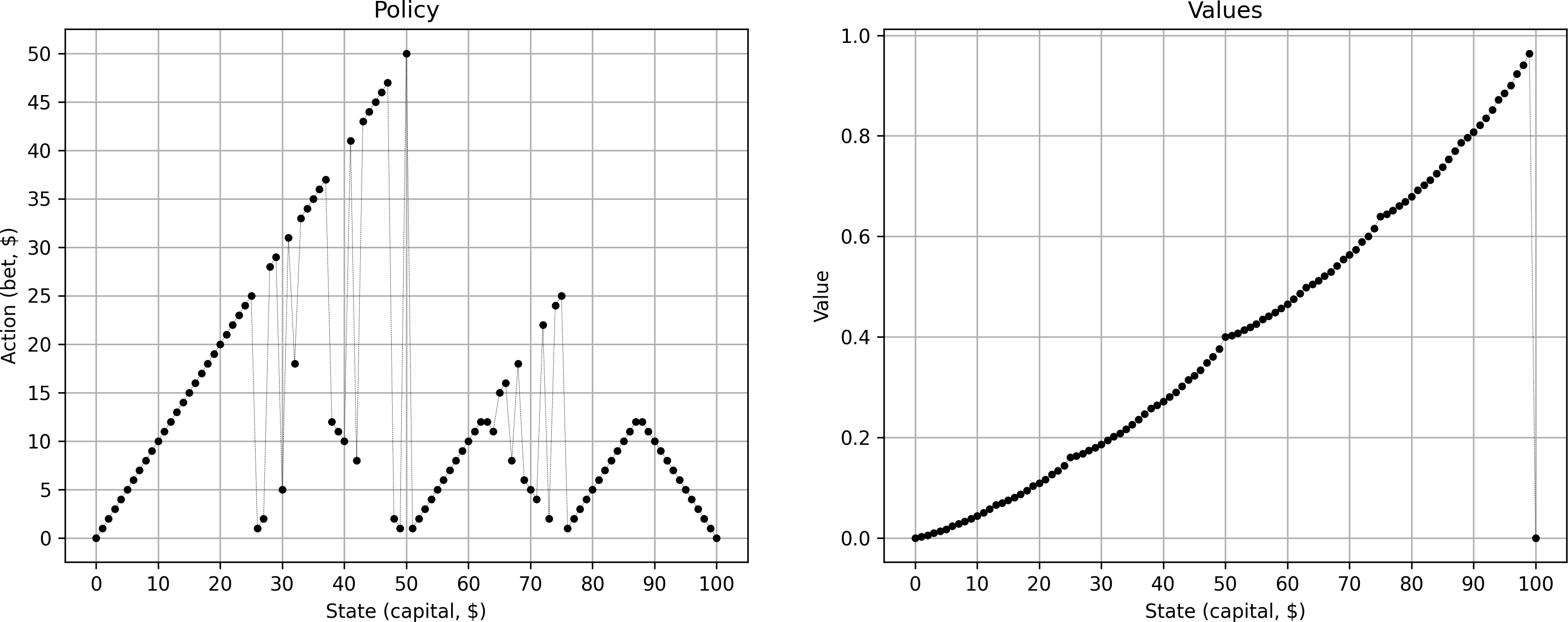
However, the policy is still very noisy. So, I started to play around with things. What if we instead update the value/policy also at equality?
-                if new_value > values[state]:
+                if new_value >= values[state]:
                     # we have found a better value/policy
                     values[state] = new_value
                     policy[state] = action
This gives me yet another policy, however, equally noisy as the previous one.
Clearly, we need to handle ties between equally good policies much more carefully. Intuitively, the gambler has a choice: If faced with equally good options, should he prefer to take the highest or lowest possible bet (or anything in between)? In other words, should he be maximally optimistic or maximally pessimistic?
Let's add a parameter optimistic - if True, the gambler will always prefer the policy with the highest bet, if False always the one with the lowest bet. Since the values are going to be very close, we also need to use np.float64 precision. This gives us the following new code:
P_HEAD = .4            # unfair coin
DISCOUNT_FACTOR = 1.0  # we choose not to discount future rewards
NUM_STATES = 101       # we include both 0 and 100 as states
THETA = 1e-9           # convergence threshold
OPTIMISTIC = False     # whether to prefer high bets
TOLERANCE = 1e-10      # tolerance for float equality

VERSION = 1

def main():
    values = np.zeros(NUM_STATES, dtype=np.float32)
    policy = np.zeros(NUM_STATES, dtype=np.int32)
    it = 0
    while True:
        it += 1
        delta = 0
        for state in range(NUM_STATES):
            if state in [0, 100]:
                # these states are terminal, i.e. we don't optimize them
                continue
            possible_actions = range(1, min([state + 1, 100 - state + 1]))  # gives e.g. [1, ..., min(s, 100 - s)]
            old_value = values[state]
            action_values = []
            for action in possible_actions:
                # we compute the value sum over all possible state transitions (i.e. throwing head or tail)
                # 1. case: head
                head_state = state + action  # we win our stake
                assert head_state <= 100
                head_reward = 1 if head_state == 100 else 0  # only give +1 reward in case of reaching $100
                head_val = P_HEAD * (head_reward + DISCOUNT_FACTOR * values[head_state])
                # 2. case: tail
                tail_state = state - action  # we lose our stake
                tail_reward = 0  # reward will always be zero
                assert tail_state >= 0
                tail_val = (1 - P_HEAD) * (tail_reward + DISCOUNT_FACTOR * values[tail_state])
                new_value = tail_val + head_val
                action_values.append((action, new_value))

            # Find global best value
            max_value = max(val for _, val in action_values)
            values[state] = max_value

            # get best actions that are very close to global best policy
            best_actions = [action for action, val in action_values if abs(val - max_value) < TOLERANCE and action > 0]
            if OPTIMISTIC:
                policy[state] = max(best_actions)
            else:
                policy[state] = min(best_actions)
            # keep track of largest diversion from original value
            delta = max(delta, abs(old_value - values[state]))

        print(f'Iteration: {it:>02}: Delta {delta:.9f}')
        if delta <= THETA:
            break
This converges in 17 iterations and FINALLY gives us the iconic plot
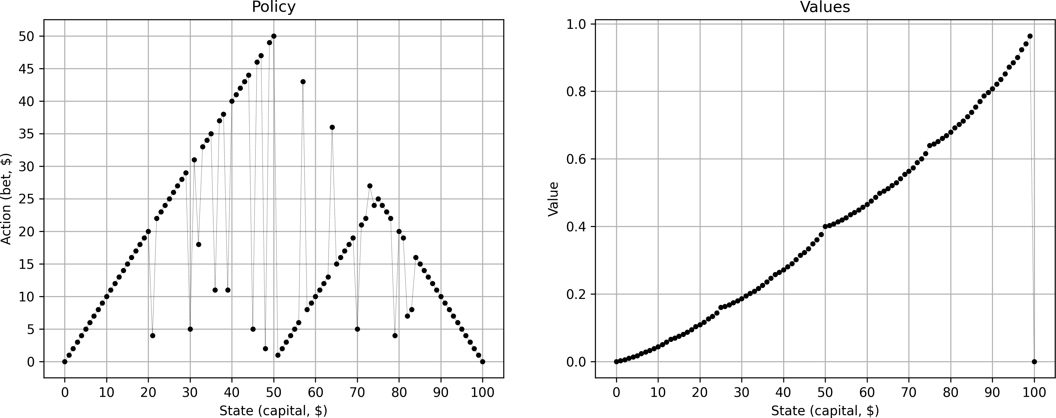
But this pattern only appears for the pessimistic case. For the optimistic case I get a simple triangle:
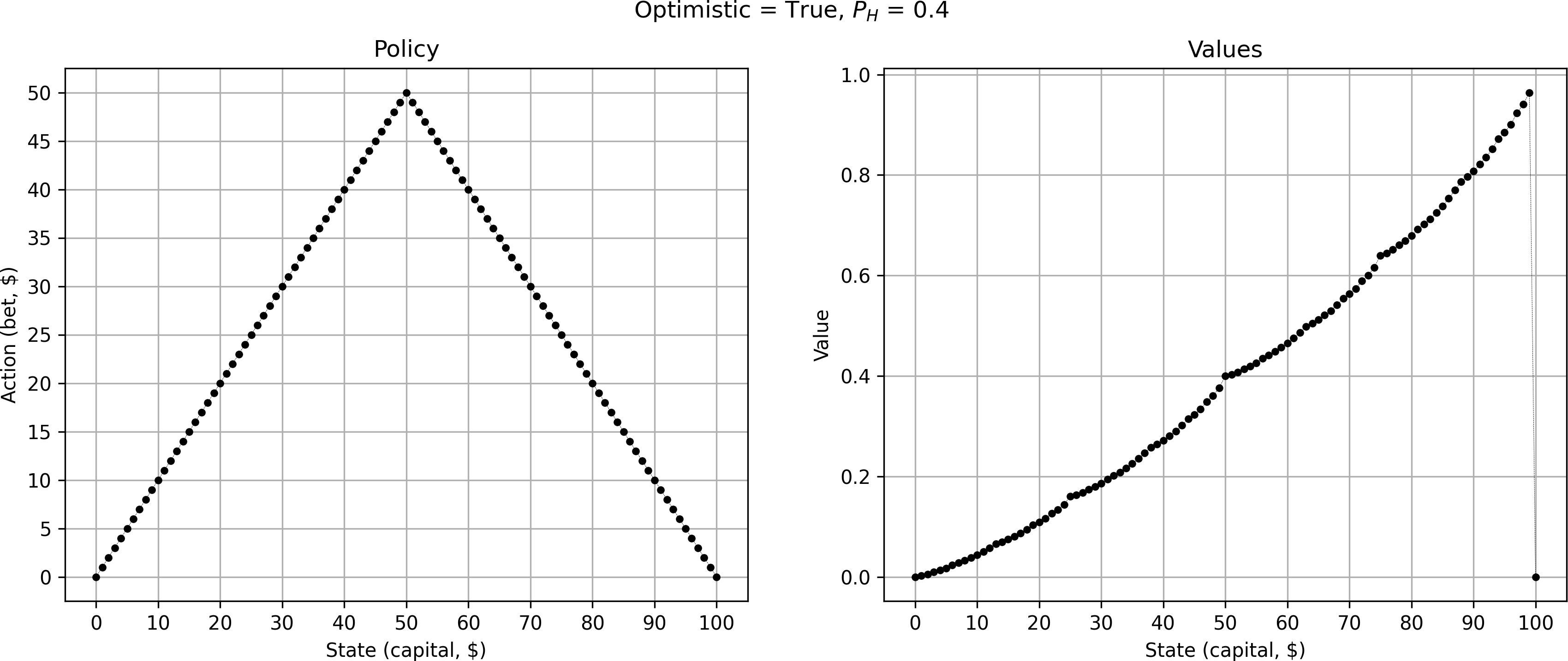
Note that both the optimistic and pessimistic case are equally optimal. Therefore, it is a perfectly viable strategy to always bet the maximum available capital (optimistic case).
Diving deeper
First, let's look at coins of different “fairness”.
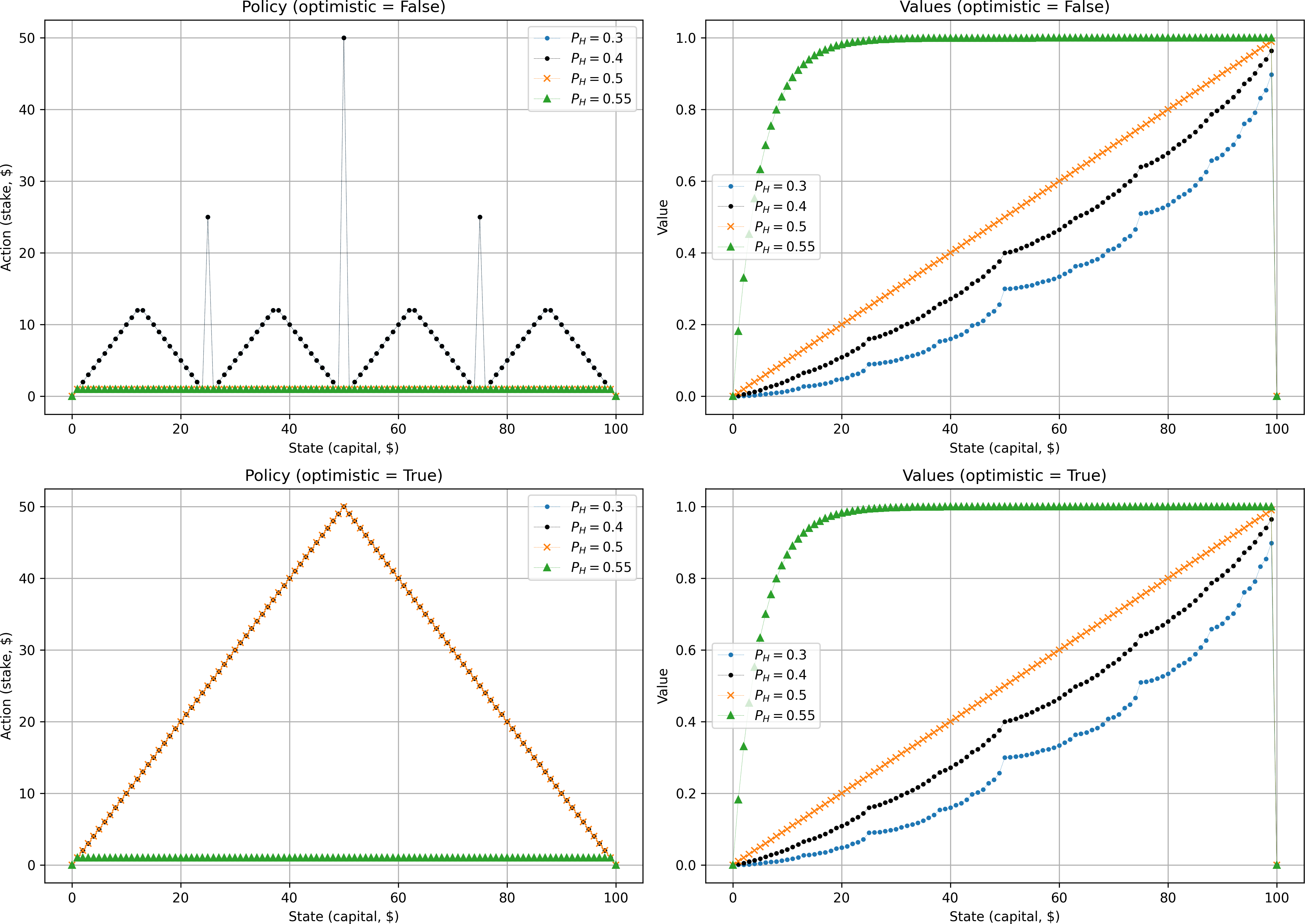
Interestingly, both unfair (blue and black) coins share identical policies (the markers are overlapping). Their respective value functions follow the same characteristic trend. The more unfavorable the coin, the lower the total expected reward. Especially for states with low levels of capital, the situation seems fairly hopeless. On the other hand, for the coin that is biased in our favor (green) the expected reward shoots up quickly and then flattens out to an almost guaranteed win after state $25. Here, the gambler always prefers to make the most cautious bet of $1 — in the long run the gambler knows that the odds are in their favor and making high bets is just taking unnecessary risks.
Let's return our focus to the original case of #(p_H = 0.4)#. So far, we've only looked at the extreme cases of optimistic or pessimistic play. Let's now visualize all optimal policies for #(p_H = 0.4)#. This gives us a neat fractal pattern, revealing some additional solutions between the optimistic and pessimistic cases above.
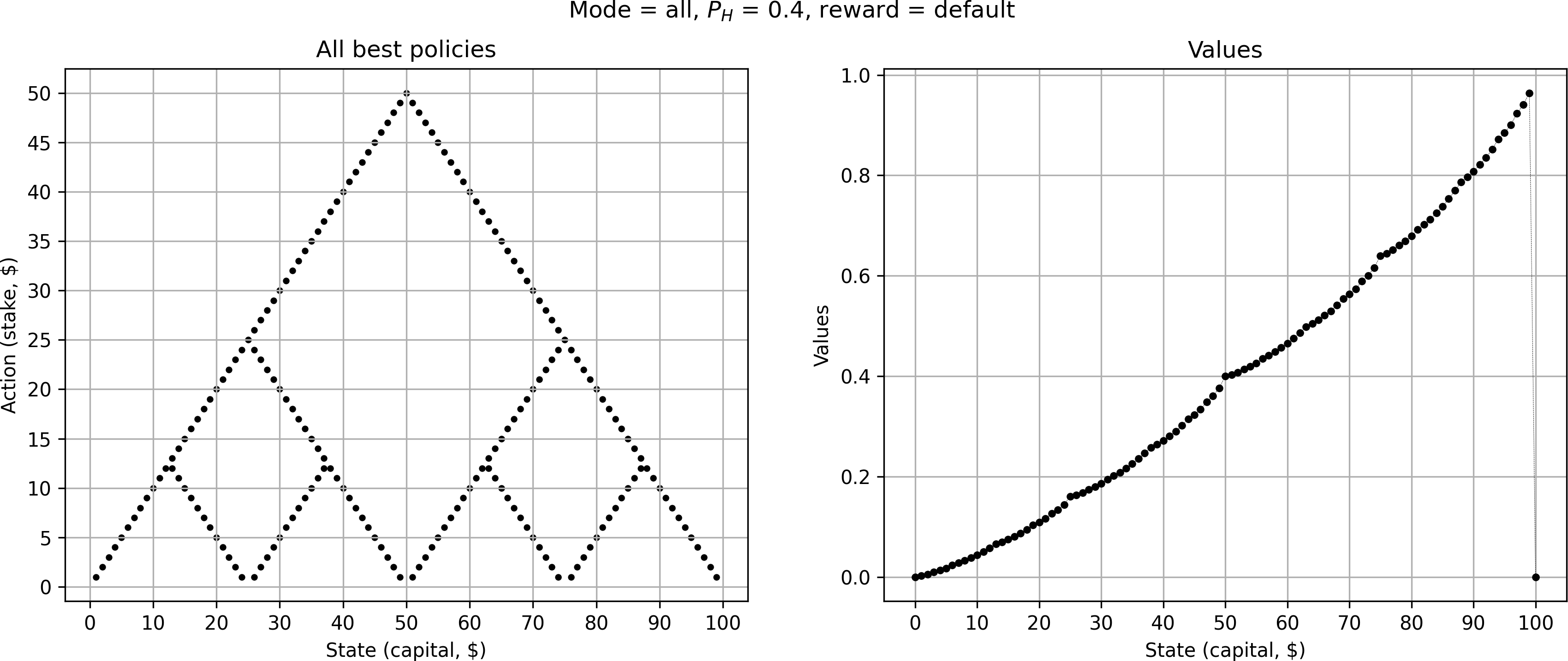
What causes this fractal pattern? Because the coin is unfair, it intuitively makes sense that we want to avoid prolonging the game unnecessarily as the odds are stacked against us. Hence, the algorithm favors policies that make fewer bets if possible. Going all-in is therefore always one of the optimal choices to make (visualized above by the ”optimistic” case). But sometimes making smaller bets can still be optimal if they put us on a path towards one of the beneficial strategic states from where we will try to leapfrog to a win.
To me it still seemed somewhat surprising that making smaller bets still leads to an optimal strategy. Maybe the gambler is just not concerned enough about running out of cash, as the reward for losing the game is 0, the same as most actions. What if we punished the gambler with a negative reward of -1 for losing the game, 0 for a non-winning action, and still +1 for winning $100?
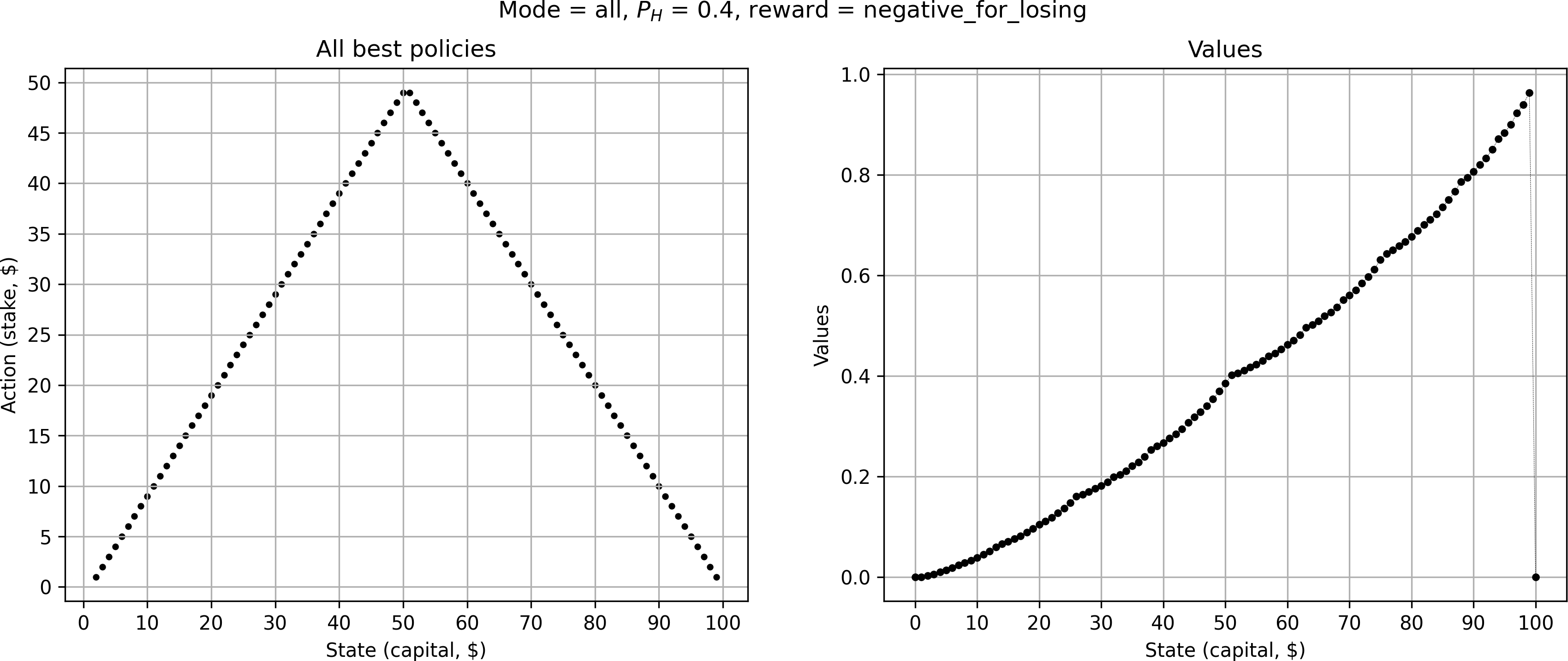
Surprisingly, this collapses the optimal policy into a single solution — and at first glance it appears to be identical to the “optimistic” triangle-like solution from before, i.e. always going all-in. Upon closer inspection, however, we notice that e.g. for a stake of $10, the gambler only bets $9 instead of all $10. Likewise, at $50 they now bet $49. Then, as soon as the gambler reaches a capital above $51, they try to go for $100 in one bet. The gambler is now much more concerned about losing the game, and as such avoids bets that risk losing the game.
Conclusion
By changing the reward function only very slightly we've completely changed the optimal policy. This shows that the original fractal pattern above is merely a consequence of a unique (and somewhat arbitrary) problem setting. The sensitivity to the exact choice of reward functions is unfortunately quite common in reinforcement learning. Nevertheless, I found it to be an eye-opening example — one that also involved a somewhat tricky implementation.
Sutton, R. S., & Barto, A. G. (2018). Reinforcement learning: An introduction. MIT press. ↩︎